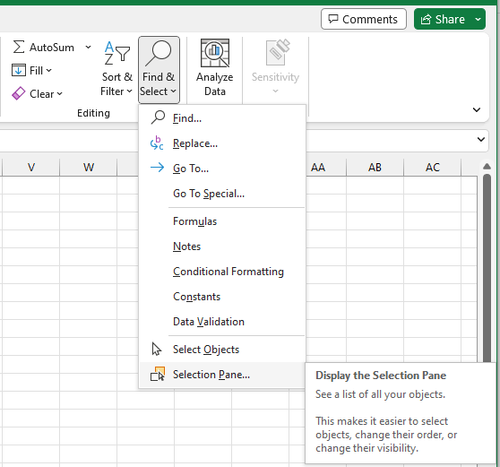
The Only Guide to Excel Links Not Working

All About Excel Links Not Working

It's easy to have several tables of data on a solitary worksheet. Formulas that are embedded in the table likewise increase as well as get with the data. An alternate method is to utilize an entire column reference, for instance. This recommendation returns all the rows in Column A. Consequently, you can include as much data as you desire, as well as the reference will always include it.


Nevertheless, range computation features like either can not handle whole column referrals or calculate all the cells in the column. User-defined functions do not instantly identify the last-used row in the column and also, therefore, frequently compute entire column references inefficiently. Nonetheless, it is easy to program user-defined features so that they acknowledge the last-used row (excel links not working).


In Excel 2007 and also later versions, range solutions can take care of whole-column recommendations, but this pressures estimation for all the cells in the column, consisting of vacant cells. This can be slow-moving to calculate, specifically for 1 million rows. By making use of the or and also features in the interpretation of a named range, you can make the area that the named variety refers to dynamically expand as well as contract.

The Best Strategy To Use For Excel Links Not Working

Utilizing the formula for a dynamic variety is normally preferable to the formula due to the fact that has the disadvantage of being an unstable feature that will be determined at every recalculation. Efficiency reduces due to the fact that the feature inside the vibrant array formula need to analyze lots of rows. You can decrease this efficiency decline by storing the part of the formula in a different cell or specified name, and afterwards describing the cell or name in the dynamic array: Counts!z1=COUNTA(Sheet1!$A:$A) Offset, Dynamic, Variety=OFFSET(Sheet1!$A$ 1,0,0, Counts!$Z$ 1,1) Index, Dynamic, Variety=Sheet1!$A$ 1: INDEX(Sheet1!$A:$A, Counts!$Z$ 1+ROW(Sheet1!$A$ 1) - 1,1) You can additionally utilize functions such as to construct dynamic ranges, but is volatile as well as always computes single-threaded.


Making use of several dynamic ranges within a single column requires special-purpose checking features. Using lots of vibrant varieties can lower efficiency. In Office 365 variation 1809 and also later on, Excel's VLOOKUP, HLOOKUP, and also suit for precise suit on unsorted information is much faster than ever when looking up multiple columns (or rows with HLOOKUP) from the very same table array.


If you make use of the precise suit alternative, the computation time for the feature is symmetrical to the number of cells checked prior to a suit is found. Lookup time utilizing the approximate match alternatives of,, as well as on arranged information is fast as well as is not dramatically boosted by the size of the range you are looking up.

The smart Trick of Excel Links Not Working That Nobody is Discussing

Make sure that you recognize the match-type and range-lookup choices in,, as well as. The complying with code instance shows the phrase structure for the function. SUIT(lookup value, lookup selection, matchtype) returns the largest match much less than or equivalent to the lookup worth when the go now lookup array is arranged rising (approximate suit).


The default choice is approximate suit arranged ascending. requests a specific suit and also assumes that the data is not sorted. returns the smallest suit better than or equal to the lookup worth if the lookup array is arranged descending (approximate match). The complying with code example shows the phrase structure for the and features.


VLOOKUP(lookup value, table range, col index num, range-lookup) HLOOKUP(lookup value, table array, row index num, range-lookup) returns the biggest suit less than or equal to the lookup worth (approximate match). Table variety have to be arranged ascending.

Getting My Excel Links Not Working To Work

If your data is sorted, yet you want an exact suit, see Usage 2 lookups for arranged data with missing values. Attempt using the as well as functions rather than. Is slightly faster (roughly 5 percent much faster), less complex, and makes use of much less memory than a combination of and also, or, the added flexibility that and also offer often allows you to significantly conserve time.


The function is fast as well as is a non-volatile function, which speeds up recalculation. The Visit Your URL feature is additionally fast; nevertheless, it is an unstable function, and it occasionally dramatically enhances the time taken to refine the estimation chain.$A$ 2:$F$ 1000, SUIT(A1,$A$ 1:$A$ 1000,0),3) Since precise match lookups can be slow, think about the adhering to options for boosting performance: Use one worksheet.


When you can, the information initially (is fast), and also make use of approximate suit. When you have to utilize a specific suit lookup, limit the array of cells to be checked to a minimum. Usage tables as well as structured recommendations or vibrant range names as opposed to referring to a big number of rows or columns.

More About Excel Links Not Working

Two approximate matches are significantly faster than one exact match for a lookup over greater than a few rows. (The breakeven factor is concerning 10-20 rows.) If you can arrange your data but still can not utilize approximate suit because you can not make certain that the worth you are searching for exists in the lookup variety, you can use this formula: IF(VLOOKUP(lookup_val, lookup_array,1, Real)=lookup_val, _ VLOOKUP(lookup_val, lookup_array, column, True), "notexist") The very first component of the formula functions by doing an approximate lookup on the lookup column itself.


VLOOKUP(lookup_val, lookup_array, column, Real) If the response from the lookup column did not match the lookup worth, you have a missing worth, and the formula returns "notexist". Understand that if you search for a worth smaller sized than the tiniest value in the checklist, you obtain an error. You can manage this mistake by utilizing, or by including a little examination worth to the checklist.


Beginning with Excel 2007, you can utilize the function, which is both basic and fast. IF IFERROR(VLOOKUP(lookupval, table, 2 FALSE),0) In earlier versions, a simple yet sluggish means is to make use of a feature which contains 2 lookups. IF(ISNA(VLOOKUP(lookupval, table,2, FALSE)),0, _ VLOOKUP(lookupval, table,2, FALSE)) You can stay clear of the double exact lookup if you make use of specific once, go to website store the outcome in a cell, and after that check the outcome prior to doing an.